Introduction to Natural Language Processing

Converting words to data

Jan 8, 2023

Cardinal Numbers

I’ll start with the wage dataset that you’ll find in an intro to econometrics textbook. We have the worker’s weekly wage, years of education, years of experience, hours worked per week, and age. Each row represents a different worker, and each column contains one piece of information about that worker. This data is old, by the way, so don’t draw any conclusions from it.

I chose to start with this dataset because it includes the most intuitive type of data: numeric cardinal data. “Cardinal” means that the numbers represent comparable quantities. A person with 20 years of experience has twice as much experience as someone with only 10 years. This differs from ordinal data, where the numbers merely indicate a ranking (e.g., a 1-5 level of satisfaction on a survey.) With cardinal data, we can visualize the relationship via a scatterplot and line of best fit.

We can represent the line via the y=mx+b format you remember from high school. For the scatterplot above, that line is:

wage = 147 + 60educ

For someone with 0 years of education, we would expect a weekly wage of $147. Furthermore, every year of education is associated with a $60 increase in one’s wage.

With more than two variables, we can’t visualize the relationships. Thus, we rely on a multi-dimensional version of the y=mx+b:

wage = -475 + 71educ + 12exper + -2hours + 13age

The constant refers to the value we’d expect if all other variables were 0. For someone with 0 years of education, 0 years of experience, working 0 hours a week, and 0 years old, we’d expect a wage of -475 per week. Yes, this doesn’t make practical sense, but the edge cases of linear regression are a topic for another day.

The other figures represent the effect on wages with all other variables held constant. All else equal, an extra year of experience is associated with an extra $12 per week, and an extra hour worked per week is associated with $2 less per week. Again, don’t draw any real-world conclusions from this data. I’m just using it to illustrate how easy it is to analyze the relationship between cardinal variables.

Bag of Words

Let’s do this one piece at a time. To start, we can remove punctuation marks. We need punctuation for grammatical reasons, but it doesn’t provide any information:

I walked the dogs and the roosters were crowing

Next, we can remove “stop words.” These are words that (like punctuation) we use for grammatical purposes, but they don’t add any meaning to the sentence. In English, these include articles like “the” and “a,” conjunctions like “and” and “or,” and various forms of the word “be.”

Specific use cases might require additional stop words. For example, when I analyze survey data at my job, I remove my company’s name from the dataset. Every review is about the company, so the name is redundant. I’m going to remove the pronoun “I” for similar reasons: all the reviews will represent the perspective of the person who wrote them.

walked dogs roosters crowing

We’re close now, but there’s still some cleaning to do. Let’s look at the word “dogs.” This word contains two parts: the base word (“dog”) and the standard English plural inflection (“s”). One sentence might mention “dog” while the other mentions “dogs.” Absent any further manipulation, our analysis would treat these as different words. Since they refer to the same concept, however, we probably don’t want that distinction. The same logic applies to “walked.” That consists of the base word “walk” and the standard English past-tense inflection “ed.” Thus, we want to “lemmatize” each work, or reduce them to their bases. This leads to:

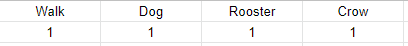
walk dog rooster crow

With that, we can create dummy variable columns.

Consider a second data point: “A cat hissed at me.” Remove stop words and convert everything to the base word, and we get “cat hiss.” Here’s what our two data points look like now:

We’ve now converted two sentences that look nothing like data into something that looks like a normal, numeric dataset. Note that we could specify the columns in one of two ways. We can make the variables binary: 1 if the statement includes the word and 0 if it doesn’t. The column could also show the number of instances of that word. For example, a sentence that included the word “dog” three times would show a “3” in the respective column.

Imagine that these sentences correspond to reviews, in which volunteers rate their satisfaction on a 1-10 scale. We can now run the same linear regression model that we used for the wage data. Consider this fabricated data:

Linear regression output might look something like this

satisfaction = 6 + 1.2dog + 0.7cat + -0.3hiss + -0.8cage

All else being equal, the mention of the “dog” in a review is associated with 1.2 additional points of satisfaction. For the word “hiss,” the figure is -0.3.

TF-IDF (Term Frequency - Inverse Document Frequency)

In the first section, we mentioned “stop words,” which occur in numerous sentences and provide no information. To add to that idea, there might be other words that are “stoppy.” We have some reason to track them, but they might occur too frequently to make any grand conclusions. For this, we can “weigh” each word by the inverse document frequency (IDF). Let’s say we have 100 reviews, and the word “dog” occurs in 80 of them. The document frequency would be 80/100. Thus, the inverse document frequency would be 100/80 or 1.25. In practice, we usually log this inverse frequency in order to deflate the value of common words and inflate the value of uncommon ones.

If a review mentions the word “dog” 5 times, and 80 out of 100 reviews mention the word dog, it will receive a value of

[Term Frequency] * [Inverse Document Frequency]
[5] * [log(100/80)]
0.48

Consider a second review that mentions “rooster” 5 times, with only 2 out of 100 reviews containing that term.

[Term Frequency] * [Inverse Document Frequency]
[5] * [log(100/5)]
6.5

I don’t see a use case for TF-IDF in linear regression. I’m not sure how one would interpret the coefficients. However, search and retrieval systems rely on the algorithm, as it allows users to find more relevant results (i.e., it doesn’t help to highlight the documents/results that use common words.)

Limitations

Both the bag of words and TF-IDF methodologies eliminate a lot of the nuance in the text. Consider the word “crow.” In our example, that was a verb referring to cock-a-doodle-doo-ing. In other instances, that same value might refer to the annoying bird. We might be able to catch some of these instances by adopting an alternative word-trimming process, like stemming. I won’t discuss the details here, but it’s a method that might work better for other texts. These methods also won’t differentiate words with multiple meanings, and they won’t account for complexities like sarcasm and idioms.

An alternative method can help us capture phrases. For these cases, we can adopt an “n-grams,” which looks at strings of N words. Consider the phrase “German Shephard.” In the “walk dog rooster crow” example, we can set n=2 and obtain the phrases “walk dog,” “dog rooster,” and “rooster crow.” The first and third show how the n-gram method can capture meaningful phrases, while the second show how the method can also pick up some nonsense. To obtain even more nonsense, we can set n=3. That produces “walk dog rooster” and “dog rooster walk,” both of which highlight the difficulties in analyzing textual data.

Word Embeddings

Word embeddings map each word to a set of numeric values. This works similarly to other unsupervised algorithms, which take something complex and reduce it to a smaller number of cardinal features. My go-to example for this is the Big Five Personality model. The statistician starts with a dataset of hundreds of answers and simplifies it to five digestible factors.

The idea behind word embeddings is that each word contains a complex set of information that one can boil down into numeric values. Consider the words “king,” “queen,” and “prince.” The words “king” and “queen” only differ with respect to sex. The words “prince” and “king,” represent the same sex, but they indicate a different level of power. All three words usually represent something usually human, though we see non-human royalty in fantasy and folklore. As such, we could “map” each word in the following way:

This royalty example represents a theoretical exercise. In practice, analysts rely on black box methodologies (usually neural networks), to perform the mapping for us. Unfortunately, neural networks lack intuitive interpretations. I can explain the linear regressions shown in earlier sections, but neural networks rely on a lot of “trust me, bro.” The practitioner might map words onto 30+ dimensions, and it’s probably not clear what any of them mean. You end up with a mystery dataset like this:

I hope that all made sense (except the neural network thing, those never make sense). At the very least, you now know more about natural language processing than whoever made this crap:

Natural Language Processing (NLP) for Machine Learning | Encora

I made up the state variable, don’t look for it in the original dataset!

I didn’t bother running an actual regression on this data, I’m just showing how it would be interpreted

Simplify